Selecting sample size for A/B testing - controlling for false positives and false negatives

Aim & key result

There are a number of online and software tools to select sample size for A/B testing. However, they tend to be black boxes with very top level insights. This prevents experimenters from truly understanding what’s going on. In this document, I give a brief introduction of what A/B testing is used for, and focus on providing a simple, yet more detailed intuition of the statistical logic.

For most practical cases, standard values for confidence and power can be used, and this yields the very practical formula below. When a power of 80% (i.e. =20%false negative rate) and a confidence level of 95% (i.e. =5%false positive rate) are chosen, and when the control and test groups are of the same size, the two tailed test is:

$$n \ge 15.7 (\sigma/\Delta)^2$$

with n the sample size needed, the estimated standard deviation and the minimal effect size that should be detected ( and should have the same units).

Full derivation and explanation of this formula and others below.

This notebook is the first part of a larger series on A/B testing mathematics:

1. A/B test sample size: statistical significance and power analysis (derivation for strong fundations - frequentist)
   • (this post)

1. A/B testing: communicating uncertainty and modelling prior knowledge (bootstrap and bayesian probabilities)

   • https://rugg2.github.io/AB%20testing%20mathematics%20-%20part%20two.html

2. A/B testing: explore vs exploit - online learning algorithms, e.g. epsilon gready & Bayesian

   • (coming soon)

Document structure

1. Problem Statement and parameters
   • what are we talking about
2. Calculating sample size - result overview
   • formulas
3. DERIVATION
   • the real meat of the document: step by step explanation of the power calculation for sample size

External resources

This is by no mean a substitute to external resources. Here are a few good ones to read after or in parallel of this document, e.g.:

• https://blog.twitter.com/engineering/en_us/a/2016/power-minimal-detectable-effect-and-bucket-size-estimation-in-ab-tests.html
• https://en.wikipedia.org/wiki/Power_(statistics)
• http://www.robotics.stanford.edu/~ronnyk/2009controlledExperimentsOnTheWebSurvey.pdf
• https://en.wikipedia.org/wiki/Sample_size_determination#Estimating_sample_sizes

Problem statement and parameters

Problem statement A/B tests are controlled experiments where some users are shown a ‘test’ version and others a ‘control’ version. The aim is to know whether the test is better, equal or worse than the control. Depending on the objective, different groupings exist:

(H0): test is similar or worse than control, (Ha): test is better than control.

• this implies using a one tailed distributions
• $\alpha$ is used for the chosen side
• for a detection threshold $\Delta>0$ (‘effect size’), this can be written $(H_a): \mu_b = \mu_a + \Delta$

(H0): test and control are similar, (Ha): test and control are different, either with test better than control or worse

• This implies using a two tailed distributions
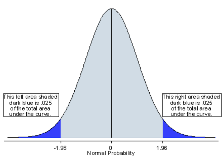
• $\alpha/2$ is used for each side
• for a detection threshold >0(‘effect size’), this can be written $(H_a):|\mu_b-\mu_a| \ge \Delta$

Business problem The question is how many samples to use / how long to run the experiment for, to avoid wasting resources but still have sound data upon which to make a good decision.

Parameters that need to be chosen

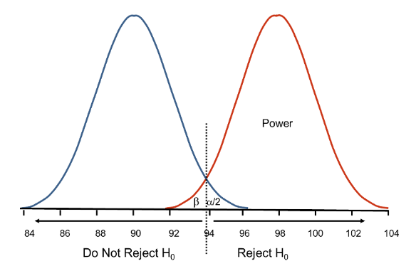
• significance / confidence level = P(keep H0 | H0 is true). It is the complementary of the probability of false positive (confidence = 1 - alpha) - i.e. how often we are willing to over-interpret noise. People often use 90-95%. Alpha = P(reject H0 | H0 is true)
• power = P(reject H0 | Ha is true). Power is about sensitivity. Power is the complementary of the probability of false negative (beta), which is how often we are willing to miss a real effect. Power = 1-beta. Beta = P(reject Ha | Ha is true). People often use Power = 80-95%
• minimum effect to be detected: $\Delta$ = AVG Performance B - AVG Performance A, or the normalised version $\Delta$ = AVG Performance B / AVG Performance A - 1, where typically B could be the test / treatment and A would be the control.

Parameter measured STandard Deviation (STD) or Standard Error (SE) : in this instance, it is probably estimated from similar experiments or it is the standard deviation of the control / default, and measured as the experiment goes on. Standard deviation gains to be smaller, so removing unnecessary noise from the experiment will make give significant results faster.

Calculating sample size - result overview

If

• a power of 80% is chosen (20% false negative rate)
• a confidence level of 95% is chosen (5% false positive rate)
• the control and test are both subject to the same sample size

then for two tailed problems (test whether the test is better or worse than control - chose this one in case of doubt):

$$n \ge 15.7 (\sigma/\Delta)^2$$

and for one tailed problems (test only whether the test is better than control, not if it is worse): $$n \ge 6.18 (\sigma/\Delta)2$$

where:

• $\sigma$ is the standard deviation of the control c and test t. If the two standard deviations are very different, $\sigma = \sqrt{(n_c \sigma_c^2 + n_t \sigma_t^2)/(n_c+n_t)}$ for samples of size $n_c$ and $n_t$.
• $\Delta$ is the amount of change you want to detect. This can be seen as the inverse of sensitivity. If you are trying to measure a revenue increase in %, you may decide that anything below $\Delta = 2%$ is not worth your time. This could also be an absolute number, e.g. control produces an average of \$100k and you will implement the test feature if it produces at least an average of \$105k: in this case $\Delta = \$5k$. It is important that $\sigma$ and $\Delta$ share the same unit / are calculated on the same thing. The smaller $\Delta$, the harder it is to differentiate between signal and noise, and therefore the higher the sample size needed.
• $n$ is the sample size needed / predicted to reach 80% power and 95% confidence level, given the standard deviationand the sensitivity

Note that $\Delta / \sigma$ is also called Cohen’s d when \$sigma$ is estimated from the standard deviation of both groups. Think of it as a normalised effect size.

As we will show, the full formula for two tailed tests is:

$$n \ge 2 \Big(\frac{\Phi^{-1}(1-\alpha/2)+\Phi^{-1}(1-\beta)}{\Delta/\sigma}\Big)^2$$

with $\Phi(x)$ the cumulative standard normal distribution.

DERIVATION

A step by step explanation of the power calculation for sample size

Quick background - law of large numbers and central limit theorem Let {X1, X2 , ... , Xn} be a sequence of independent and identically distributed (i.i.d.) random variables drawn from a distribution of expected value and a finite standard deviation . We are interested in the sample average $\bar{X}_n= (X_1 + ... + X_n) / n$.

By the law of large numbers , the sample average converges to the expected value $\bar{X}_n \to \mu$ when $n \to \infty$. Coming back to our A/B test, we’ll have $A_n \to A$ and $B_n \to B$ as the sample size n becomes big, which means that we’ll ultimately know the true mean of A and B given enough samples. The question is how many samples are enough to be confident that $\mu_A > \mu_B$ or $\mu_B > \mu_A$.

One way to start estimating this is to look at the variance. As a reminder, the variance is the square of the standard deviation $Var(x_1) = STD(x_1)^2 = \sigma^2$. For two independent variables Y and Z, Var(Y+Z) = Var(Y) + Var(Z). Also, for a constant a, Var(a Z) = a^2 Var(Z). As X1 and X2 are i.i.d., Var(X1) = Var(X2). This means that:

$$Var(\bar{X}_n) = Var(1/n \, \sum_{i=1}^{n} \, X_i) = \sum_{i=1}^{n} \, Var(1/n \, X_i) = n \, Var(1/n X_1) = n \, (1/n)^2 \, Var(X_1) = \sigma^2/n$$

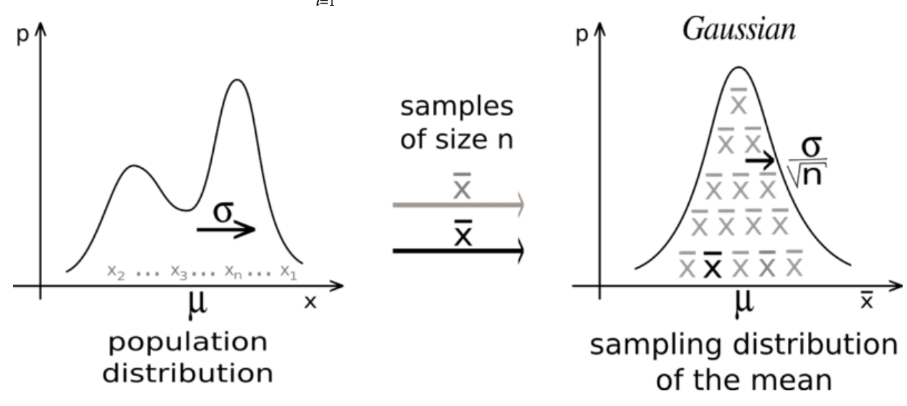
This can be rewritten as the standard error of the mean (SEM) being smaller than the standard error of our variables $X_i: SEM =STD(\bar{X}_n) = STD(X_1)/\sqrt{n} = \sigma/\sqrt{n}$. So multiplying the sample size by 4 will reduce the fluctuations in the means estimate by 2.

Although this gives us quite a bit of information about how the means fluctuates, with X having an unknown distribution, we cannot really estimate the probability of two estimated means $A_n$ and $B_n$ being truly different vs being the effect of natural fluctuations. This is where the central limit theorem gives us some pretty amazing results: for almost all distributions the normalized sum of iid variables tends towards a normal distribution!

$$ \bar{X}_n = 1/n \, \sum_{i=1}^{n} x_i \sim N(\mu, STD(\bar{X}_n)) = N(\mu, \sigma/\sqrt{n})$$

For the rest of this document we will assume that the sample size is large enough that the sample means behaves as a normal distribution. For small sample sizes, the situation can not always be resolved. If variables X were to behave as a normal distribution (with unknown standard deviation), the mean of those normal distributions follows the Student’s t-distribution. We won’t consider small sample sizes here.

Choosing sample size from significance, power and minimal effect Let us consider $X_i= B_i-A_i$, for i=1..n, and assume they are independent and identically distributed, with a known variance but an unknown mean. One potential business problem is to know whether $\mu:=\mu_B - \mu_A > \Delta$, and this is this one-tailed test that we will demonstrate, the two-tailed demonstration is very similar. We will assume that n is large enough that the central limit theorem kicks in and that the sample means behaves as a normal distribution.

Mathematically, the default hypothesis would typically be that A and B are mostly the same, and the alternative hypothesis is that there are at different by at least the minimal effect size: $$(H_0): \mu = 0$$ $$(H_a): \mu > \Delta$$

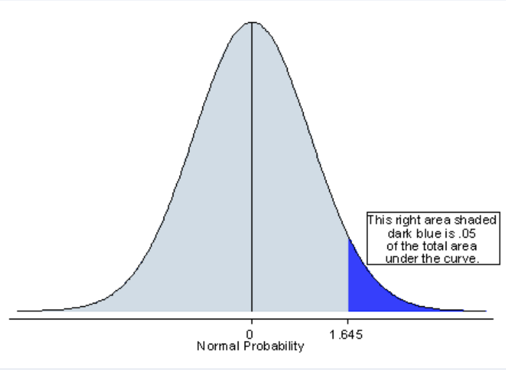
Let $\alpha$ be the false positive rate ($confidence \, level = 1 - \alpha$), and $\beta$ the false negative rate ($power = 1 - \beta$). Let $\Phi(x)$ be the cumulative standard normal distribution. Some of you may be familiar with the z notation: $\Phi^{-1}(1-\alpha) = z_{\alpha}$, the upper $\alpha$ percentage point of the standard normal distribution. This means that if Y is normally distributed, i.e. Y ~ N(0,1), then $P(Y \le x) = \Phi(x)$, and so $$P(Y>z)=\alpha \Leftrightarrow 1-\Phi(z) = \alpha \Leftrightarrow z = \Phi^{-1}(1-\alpha)$$

As we saw, for large sample sizes n, approximating the sample means to a normal distribution is pretty legit: $\bar{X}_n \sqrt{n} / \sigma \sim N(\mu, 1)$.

Controlling for false positives: P(reject H0 | H0 true) We want, assuming (H0) holds, $\mu=0$, so $\bar{X}_n \sqrt{n} / \sigma \sim N(0, 1)$ and the condition to control for false positives can be written (one tailed test):

$$P( reject \, H_0 \, | \, H_0 \, true) = \alpha$$ $$\Leftrightarrow P(\bar{X}_n \sqrt{n} / \sigma > \Phi^{-1}(1-\alpha) \, | \, H_0 \, true) = \alpha$$

Which can we verbalized as ‘reject H0 if our sample average Xn is more than $\Phi^{-1}(1-\alpha) \, \sigma / \sqrt{n}$’, for a chosen risk probability of $\alpha$, often chosen to be 0.05.

At any point in the trial we can estimate the sample size and decide whether a result is significant or not. The remaining question is when we should stop, and this is linked to the power and false negative rate.

Controlling for false negatives - P(keep H0 | Ha is true) Assuming (Ha) holds, then $\mu=\Delta$, and $(\bar{X}_n-\Delta) \, \sqrt{n} / \sigma \sim N(0, 1)$. The condition to control for the false negatives can be written (one tailed test):

$$P( keep \, H_0 \,| \,H_a \,true) \le \beta$$

As we saw, the criteria to keep H0 with a confidence alpha is $\bar{X}_n \sqrt{n} / \sigma \le \Phi^{-1}(1-\alpha)$. In practice we don’t know which hypothesis is true, so we’d apply the same criteria in both cases, and power is about the risk of it misfiring.

$$P(\bar{X}_n \sqrt{n}/\sigma \le \Phi^{-1}(1-\alpha) \,| \, H_a \, true) \le \beta$$

The twist is that $\bar{X}_n \sqrt{n} / \sigma $ does not follow a standard normal distribution N(0,1) anymore when Ha is true, it’s $(\bar{X}_n-\Delta) \sqrt{n} / \sigma$ that does. To be able to use $Phi$, we can rewrite the equation to make that term appear:

$$P\Big( (\bar{X}_n - \Delta + \Delta) \, \sqrt{n}/\sigma \le \Phi^{-1}(1-\alpha) \, | \, H_a \, true\Big) \le \beta $$

$$\Leftrightarrow P\Big( (\bar{X}_n - \Delta) \, \sqrt{n}/\sigma \le \Phi^{-1}(1-\alpha) - \Delta \sqrt{n}/\sigma \,| \, H_a \, true\Big) \le \beta$$

$$\Leftrightarrow \Phi \Big(\Phi^{-1}(1-\alpha) - \Delta \sqrt{n}/\sigma \Big) \le \beta$$

$$\Leftrightarrow \Phi^{-1}(1-\alpha) - \Delta \sqrt{n}/\sigma \le \Phi^{-1}(\beta)$$

So we can now express the sample size n as a function of alpha, beta, delta and sigma:

$$n \ge \Big( \frac{\Phi^{-1}(1-\alpha) - \Phi^{-1}(\beta)}{\Delta/\sigma} \Big)^2$$

This can also be written in terms of power, using $\Phi^{-1}(1-\beta) =-\Phi^{-1}(\beta)$ as $\Phi^{-1}$ has a ‘odd symmetry’ around 0.5 :$\Phi^{-1}(1-\beta)=\Phi^{-1}(0.5+(0.5-\beta))= -\Phi^{-1}(0.5-(0.5-\beta))= -\Phi^{-1}(\beta), so

$$P( keep \, H_0 \, | \, H_a \, true) \le \beta$$

$$\Leftrightarrow n \ge \Big( \frac{\Phi^{-1}(1-\alpha) + \Phi^{-1}(1-\beta)} {\Delta / \sigma} \Big)^2$$

Numerical example

Functions to calculate $z_{\alpha} = \Phi^{-1}(1-\alpha)$ and $\Phi^{-1}(1-\beta)$are widely available. The $\Phi^{-1}$ function is the inverse cumulative standard normal distribution, and it is also called probit function. How to get values:

• Excel / Google sheets: -1(1-) = NORMINV(1-alpha, 0, 1),
• Python:
  • from scipy.stats import norm
  • norm.ppf(1-alpha, mean=0, stddev=1)
• Some values: $\Phi^{-1}(0.95)=1.645$ ; $\Phi^{-1}(0.9)=1.282$ ; $\Phi^{-1}(0.85)=1.036$ ; $\Phi^{-1}(0.8)=0.8416$

As discussed, choosing the false positive and false negative rate is a business decision, as it is a tradeoff between more certainty and using more resources.

• A good starting point used in many cases is to chose a false positive rate =0.05and a false negative rate =0.2.
• This is equivalent to a confidence $1-\alpha =0.95$ and a power $1-\beta=0.8$

Applying the inverse cumulative standard normal distribution, we get:

• $\Phi^{-1}(1-\alpha)=\Phi^{-1}(1-0.05) = \Phi^{-1}(0.95) = 1.645$
• $\Phi^{-1}(1-\beta)=\Phi^{-1}(1-0.2) = \Phi^{-1}(0.8) = 0.8416$

This yields a sample size for power, one-tailed test ($\mu_A<\mu_B$ or more accurately $\mu_A \le \mu_B + \Delta$):

$$ n \ge \Big( \frac{\Phi^{-1}(1-\alpha) + \Phi^{-1}(1-\beta)} {\Delta / \sigma} \Big)^2 = (1.645+0.8416)^2 (\sigma/\Delta)^2=6.183 (\sigma/\Delta)^2$$

Note that, if you want to only cater for false positives, the sample size can be smaller as the $\Phi^{-1}(1-\beta)$ disappears.

If you want to conduct a two-tailed test, (if the test is $\mu_A \ne \mu_B$ or more accurately $|\mu_A-\mu_B| \ge \Delta$) this becomes:

$$ n \ge 2 \Big( \frac{\Phi^{-1}(1-\alpha/2) + \Phi^{-1}(1-\beta)} {\Delta / \sigma} \Big)^2 = 2*(1.960+0.8416)^2 (\sigma/\Delta)^2 = 15.70 (\sigma/\Delta)^2$$